Within-person factorial experiments, log(normal) reaction-time data | A. Solomon Kurz
Causal inference with the GLMM, Part 1| A. Solomon Kurz
Causal inference with the GLMM, Part 1| A. Solomon Kurz

A workshop through the VISN 17 Center of Excellence| A. Solomon Kurz
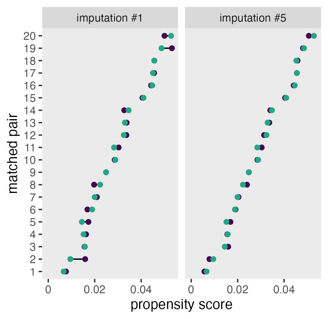
I'm finally dipping my does into causal inference for quasi-experiments, and my first use case has missing data. In this post we practice propensity score matching with multiply-imputed data sets, and how to compute the average treatment effect for the treated (ATT) with g-computation.| A. Solomon Kurz
Sometimes in the methodological literature, models for continuous outcomes are presumed to use the Gaussian likelihood. In the sixth post of this series, we saw the gamma likelihood is a great alternative when your continuous data are restricted to positive values, such as in reaction times and bodyweight. In this ninth post, we practice making causal inferences with the beta likelihood for continuous data restricted within the range of \((0, 1)\).| A. Solomon Kurz
So far in this series, we have used the posttreatment scores as the dependent variables in our analyses. However, it’s not uncommon for researchers to frame their questions in terms of change from baseline with a change-score (aka gain score) analysis. The goal of this post is to investigate whether and when we can use change scores or change from baseline to make causal inferences. Spoiler: Yes, sometimes we can (with caveats).| A. Solomon Kurz
Books At present, all of my books share a similar format and goal. I am a fan of applied Bayesian statistics. In recent years, scholars have released user-friendly Bayesian software packages and have published reasonably-accessible introductory books on applied Bayesian analysis. These have been boons for us all. In my experience, Bayesian methods are easiest to use within the R computing environment by way of Paul Bürkner’s brms package. At present, very few textbooks showcase how to use ...| A. Solomon Kurz
We social scientists love collecting ordinal data, such as those from questionnaires using Likert-type items.1 Sometimes we’re lazy and analyze these data as if they were continuous, but we all know they’re not, and the evidence suggests things can go terribly horribly wrong when you do ( Liddell & Kruschke, 2018). Happily, our friends the statisticians and quantitative methodologists have built up a rich analytic framework for ordinal data (see Bürkner & Vuorre, 2019).| A. Solomon Kurz
So far the difficulties we have seen with covaraites, causal inference, and the GLM have all been restricted to discrete models (e.g., binomial, Poisson, negative binomial). In this sixth post of the series, we’ll see this issue can extend to models for continuous data, too. As it turns out, it may have less to do with the likelihood function, and more to do with the choice of link function. To highlight the point, we’ll compare Gaussian and gamma models, with both the identity and log li...| A. Solomon Kurz
In the third post in this series, we extended out counterfactual causal-inference framework to binary outcome data. We saw how logistic regression complicated the approach, particularly when using baseline covariates. In this post, we’ll practice causal inference with unbounded count data, using the Poisson and negative-binomial likelihoods. We need data We’ll be working with a subset of the epilepsy data from the brms package. Based on the brms documentation (execute ?| A. Solomon Kurz
In the first two posts of this series, we relied on ordinary least squares (OLS). In the third post, we expanded to maximum likelihood for a couple logistic regression models. In all cases, we approached inference from a frequentist perspective. In this fourth post, we’re finally ready to make causal inferences as Bayesians. We’ll do so by refitting the Gaussian and binomial models from the previous posts with the Bayesian brms package ( Bürkner, 2017, 2018, 2022), and show how to comput...| A. Solomon Kurz
So far in this series, we’ve been been using ordinary least squares (OLS) to analyze and make causal inferences from our experimental data. Though OLS is an applied statistics workhorse and performs admirably in some cases, there are many contexts in which it’s just not appropriate. In medical trials, for example, many of the outcome variables are binary. Some typical examples are whether a participant still has the disease (coded 1) or not (coded 0), or whether a participant has died (co...| A. Solomon Kurz
One of the nice things about the simple OLS models we fit in the last post is they’re easy to interpret. The various \(\beta\) parameters were valid estimates of the population effects for one treatment group relative to the wait-list control.1 However, this nice property won’t hold in many cases where the nature of our dependent variables and/or research design requires us to fit other kinds of models from the broader generalized linear mixed model (GLMM) framework.| A. Solomon Kurz
Welcome to the beginning This is the first post in a series on causal inference. Our ultimate goal is to learn how to analyze data from true experiments, such as RCT’s, with various likelihoods from the generalized linear model (GLM), and with techniques from the contemporary causal inference literature. We’ll do so both as frequentists and as Bayesians. I’m writing this series because even though I learned a lot about data analysis and research design during my PhD, I did not receive t...| A. Solomon Kurz
⚠️ This workshop has already come and gone. You can find some of the original marketing descriptions, along with a link to the online supporting materials, below. Overview We are entering the Golden Age of Bayesian statistics. Thanks to fast personal computers and powerful free software (e.g., Stan), working scientists can fit an array of Bayesian models tailored to their specific needs. Recent textbooks from authors like McElreath (2015, 2020) have also made Bayesian methods more accessi...| A. Solomon Kurz
Courses 2022 Fall semester Statistical Analysis (PA 652) For: The Chicago School of Professional Psychology, Los Angeles Where: Online Goal: This course is designed to introduce the generalized linear mixed model (GLMM) to doctoral students in behavior analysis. We start the semester with simple regression via ordinary least squares, introduce the generalized linear model with maximum likelihood by mid semester, and end the semester with conditional longitudinal models via the full GLMM.| A. Solomon Kurz
Purpose Once again, it was time to update my website. This time I am switching to the Hugo Apéro (a-pay-ROH) theme, by the great Alison Hill. The purpose of this post is to highlight some of the steps I took to rebuild my website. At a minimum, I’m hoping this post will help me better understand how to set up my website the next time it needs an overhaul. Perhaps it will be of some help to you, too.| A. Solomon Kurz
Support Yes, you can support me Every so often, people ask how they might support the work I do with my tutorial blog posts and ebooks. Here are some options: If you like my material, give it a shout out on Twitter! You can find me there at https://twitter.com/SolomonKurz. If my material directly helped your scientific work, consider citing them. You can find tips on how to cite blog posts in APA 7 style here.| A. Solomon Kurz
What? We psychologists analyze a lot of sum-score data. Even though it’s not the best, we usually use the Gaussian likelihood1 for these analyses. I was recently in a situation were I wanted to model sum-scores from a new questionnaire and there was no good prior research on the distribution of the sum-scores. Like, there wasn’t a single published paper reporting the sample statistics. Crazy, I know… Anyway, I spent some time trying to reason through how I would set a justifiable prior ...| A. Solomon Kurz
What? All the players know there are three major ways to handle missing data: full-information maximum likelihood, multiple imputation, and one-step full-luxury1 Bayesian imputation. In an earlier post, we walked through method for plotting the fitted lines from models fit with multiply-imputed data. In this post, we’ll discuss another neglected topic: How might one compute standardized regression coefficients from models fit with multiply-imputed data? I make assumptions. For this post, I...| A. Solomon Kurz
What/why? This is a follow-up to my earlier post, Notes on the Bayesian cumulative probit. If you haven’t browsed through that post or if you aren’t at least familiar with Bayesian cumulative probit models, you’ll want to go there, first. Comparatively speaking, this post will be short and focused. The topic we’re addressing is: After you fit a full multilevel Bayesian cumulative probit model of several Likert-type items from a multi-item questionnaire, how can you use the model to co...| A. Solomon Kurz
Abstract Background: The USA is undergoing a suicide epidemic for its youngest Veterans (18-to-34-years-old) as their suicide rate has almost doubled since 2001. Veterans are at the highest risk during their first-year post-discharge, thus creating a “deadly gap.” In response, the nation has developed strategies that emphasize a preventive, universal, and public health approach and embrace the value of community interventions. The three-step theory of suicide suggests that community inter...| A. Solomon Kurz
Abstract Research on moral elevation has steadily increased and identified several psychosocial benefits that bear relevance to both the general population and people with psychological distress. However, elevation measurement is inconsistent, and few state-level measures have been created and critically evaluated to date. To address this gap, the State Moral Elevation Scale (SMES) was developed and tested using an online sample (N = 930) including subsamples of general participants (nonclini...| A. Solomon Kurz
Preamble In an earlier post, I gave an example of what a power analysis report could look like for a multilevel model. At my day job, I was recently asked for a rush-job power analysis that required a multilevel model of a different kind and it seemed like a good opportunity to share another example. For the sake of confidentiality, some of the original content will be omitted or slightly altered.| A. Solomon Kurz
Abstract Lifestyle behaviors such as exercise, sleep, smoking, diet, and social interaction are associated with depression. This study aimed to model the complex relationships between lifestyle behaviors and depression and among the lifestyle behaviors. Data from three waves of the Midlife in the United States study were used, involving 6898 adults. Network models revealed associations between the lifestyle behaviors and depression, with smoker status being strongly associated with depression...| A. Solomon Kurz
Abstract Objective: Posttraumatic stress disorder (PTSD) is a common problem for veterans. Resilience, the tendency to bounce back from difficult circumstances, is negatively associated with posttraumatic cognitions (PTCs) among individuals with a history of trauma, and thus it may be important to understand responses to trauma reminders. Methods: Using a quasi-experimental design, we examined the association between trait resilience and state PTCs in veterans with PTSD $(n = 47, M_\textit{ag...| A. Solomon Kurz
What/why? Prompted by a couple of my research projects, I’ve been fitting a lot of ordinal models, lately. Because of its nice interpretive properties, I’m fond of using the cumulative probit. Though I’ve written about cumulative logit ( Kurz, 2020b, sec. 11.1) and probit models ( Kurz, 2020a, Chapter 23) before, I still didn’t feel grounded enough to make rational decisions about priors and parameter interpretations. In this post, I have collected my recent notes and reformatted them...| A. Solomon Kurz
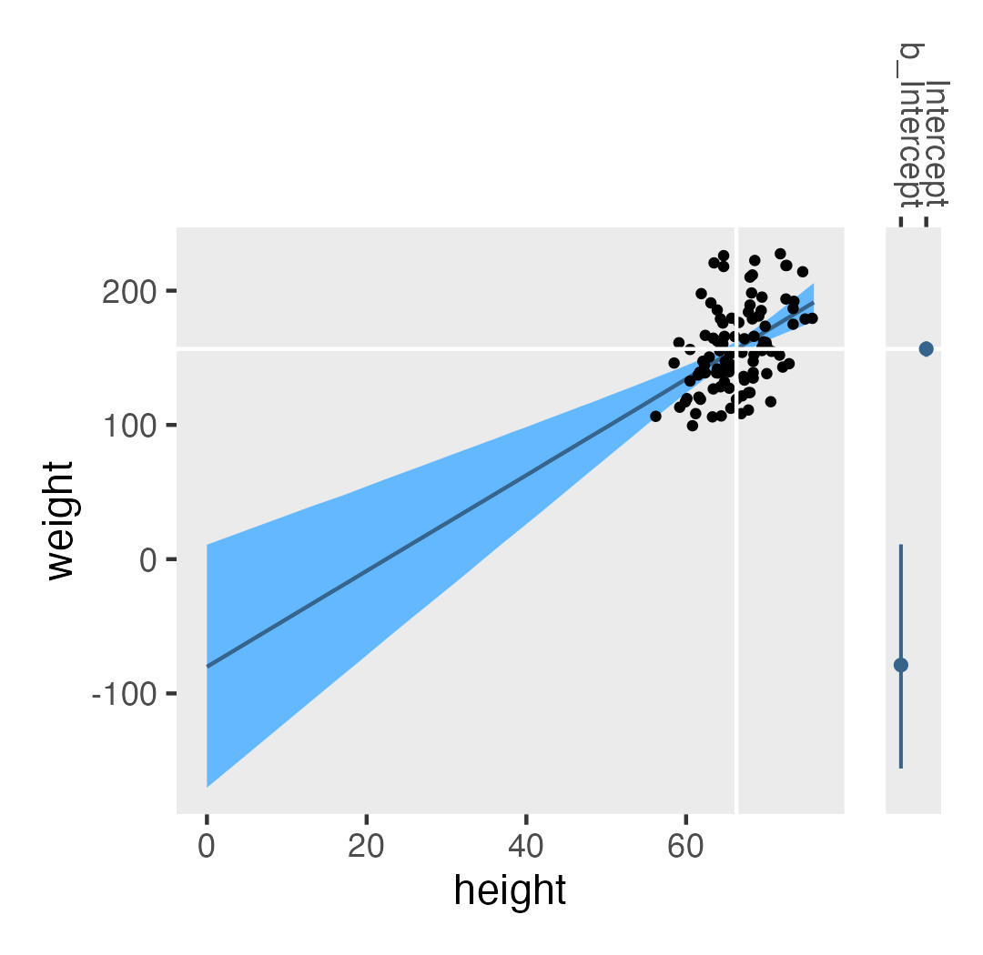
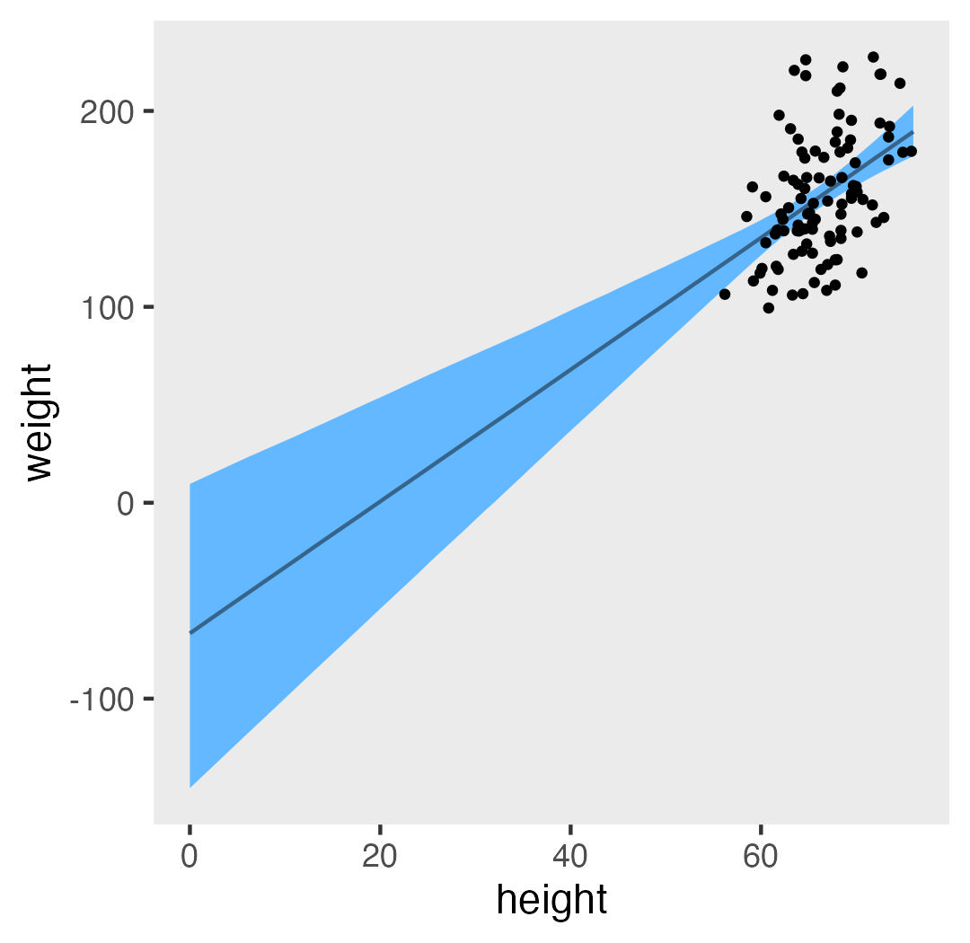
Scenario You’re an R ( R Core Team, 2022) user and just fit a nice multilevel model to some grouped data and you’d like to showcase the results in a plot. In your plots, it would be ideal to express the model uncertainty with 95% interval bands. If you’re a Bayesian working with Stan-based software, such as brms ( Bürkner, 2017, 2018, 2022), this is pretty trivial. But if you’re a frequentist and like using the popular lme4 package ( Bates et al.| A. Solomon Kurz
Version 1.1.0 Edited on December 12, 2022, to use the new as_draws_df() workflow. Preamble After tremendous help from Henrik Singmann and Mattan Ben-Shachar, I finally have two (!) workflows for conditional logistic models with brms. These workflows are on track to make it into the next update of my ebook translation of Kruschke’s text (see here). But these models are new to me and I’m not entirely confident I’ve walked them out properly.| A. Solomon Kurz
Version 1.1.0 Edited on October 9, 2022. Doctoral candidate Reinier van Linschoten kindly pointed out a mistake in my R code for \(V_B\), the between imputation variance. The blog post now includes the corrected workflow. What? If you’re in the know, you know there are three major ways to handle missing data: full-information maximum likelihood, multiple imputation, and one-step full-luxury1 Bayesian imputation. If you’re a frequentist, you only have the first two options.| A. Solomon Kurz
What When you fit a logistic regression model, there are a lot of ways to display the results. One of the least inspiring ways is to report a summary of the coefficients in prose or within a table. A more artistic approach is to show the fitted line in a plot, which often looks nice due to the curvy nature of logistic regression lines. The major shortcoming in typical logistic regression line plots is they usually don’t show the data due to overplottong across the \(y\)-axis.| A. Solomon Kurz
Abstract Although there is growing interest in the neural foundations of aesthetic experience, it remains unclear how particular mental subsystems (e.g. perceptual, affective and cognitive) are involved in different types of aesthetic judgements. Here, we use fMRI to investigate the involvement of different neural networks during aesthetic judgements of visual artworks with implied motion cues. First, a behavioural experiment \((N = 45)\) confirmed a preference for paintings with implied moti...| A. Solomon Kurz
Version 1.1.0 Edited on December 12, 2022, to use the new as_draws_df() workflow. Preamble Suppose you’ve got data from a randomized controlled trial (RCT) where participants received either treatment or control. Further suppose you only collected data at two time points, pre- and post-treatment. Even in the best of scenarios, you’ll probably have some dropout in those post-treatment data. To get the full benefit of your data, you can use one-step Bayesian imputation when you compute your...| A. Solomon Kurz
Abstract A starting point of many digital health interventions informed by the Stages of Change Model of behavior change is assessing a person’s readiness to change. In this paper, we use the concept of readiness to develop and validate a prediction model of health-seeking behavior in the context of family planning. We conducted a secondary analysis of routinely collected, anonymized health data submitted by 4,088 female users of a free health chatbot in Kenya.| A. Solomon Kurz
Version 1.1.0 Edited on December 12, 2022, to use the new as_draws_df() workflow. What? One of Tristan Mahr’s recent Twitter threads almost broke my brain. wait when people talk about treating overdispersion by using random effects, they sometimes put a random intercept on each row?? https://t.co/7NjG4uw3nz pic.twitter.com/fo8Ylcejqv — guy whose whole personality is duckdb 🦆 (@tjmahr) July 8, 2021 It turns out that you can use random effects on cross-sectional count data.| A. Solomon Kurz
Context In one of my recent Twitter posts, I got pissy and complained about a vague power-analysis statement I saw while reviewing a manuscript submitted to a scientific journal. If you submit a manuscript for publication that involves HLMs and SEMs of longitudinal data and you vaguely summarize your power analysis in one sentence, I, as your friendly neighborhood Reviewer #2, am requesting a full power-analysis write-up as a supplementary material.| A. Solomon Kurz
Version 1.1.0 Edited on December 12, 2022, to use the new as_draws_df() workflow. Context Someone recently posted a thread on the Stan forums asking how one might make item-characteristic curve (ICC) and item-information curve (IIC) plots for an item-response theory (IRT) model fit with brms. People were slow to provide answers and I came up disappointingly empty handed after a quick web search. The purpose of this blog post is to show how one might make ICC and IIC plots for brms IRT models ...| A. Solomon Kurz
tl;dr When your MCMC chains look a mess, you might have to manually set your initial values. If you’re a fancy pants, you can use a custom function. Context A collaborator asked me to help model some reaction-time data. One of the first steps was to decide on a reasonable likelihood function. You can see a productive Twitter thread on that process here. Although I’ve settled on the shifted-lognormal function, I also considered the exponentially modified Gaussian function (a.| A. Solomon Kurz
Purpose Just this past week, I learned that, Yes, you can fit an exploratory factor analysis (EFA) with lavaan ( Rosseel, 2012; Rosseel & Jorgensen, 2019). At the moment, this functionality is only unofficially supported, which is likely why many don’t know about it, yet. You can get the [un]official details at issue #112 on the lavaan GitHub repository ( https://github.com/yrosseel/lavaan). The purpose of this blog post is to make EFAs with lavaan even more accessible and web searchable by...| A. Solomon Kurz
Purpose A few weeks ago, I was preparing to release the second blog post in a two-part series (you can find that post here). During the editing process, I had rendered the files into HTML and tried posting the draft to my website. Everything looked fine except that the figures wouldn’t render. I hadn’t seen this behavior before and I figured it had to do with some software update. When I checked, the blogdown package ( Xie et al.| A. Solomon Kurz
Version 1.1.0 Edited on December 12, 2022, to use the new as_draws_df() workflow. Orientation This post is the second and final installment of a two-part series. In the first post, we explored how one might compute an effect size for two-group experimental data with only \(2\) time points. In this second post, we fulfill our goal to show how to generalize this framework to experimental data collected over \(3+\) time points.| A. Solomon Kurz
Background This post is the first installment of a two-part series. The impetus is a project at work. A colleague had longitudinal data for participants in two experimental groups, which they examined with a multilevel growth model of the kind we’ll explore in the next post. My colleague then summarized the difference in growth for the two conditions with a standardized mean difference they called \(d\). Their effect size looked large, to me, and I was perplexed when I saw the formula they ...| A. Solomon Kurz
Version 1.1.0 Edited on December 16, 2022, to use the new as_draws_df() workflow. Purpose In the contemporary longitudinal data analysis literature, 2-timepoint data (a.k.a. pre/post data) get a bad wrap. Singer and Willett ( 2003, p. 10) described 2-timepoint data as only “marginally better” than cross-sectional data and Rogosa et al. ( 1982) give a technical overview on the limitations of 2-timepoint data. Limitations aside, sometimes two timepoints are all you have.| A. Solomon Kurz
Version 1.1.0 Edited on December 16, 2022, to use the new as_draws_df() workflow. The set-up PhD candidate Huaiyu Liu recently reached out with a question about how to analyze clustered data. Liu’s basic setup was an experiment with four conditions. The dependent variable was binary, where success = 1, fail = 0. Each participant completed multiple trials under each of the four conditions. The catch was Liu wanted to model those four conditions with a multilevel model using the index-variabl...| A. Solomon Kurz
Abstract Research on moral elevation has steadily increased and identified several psychosocial benefits that bear relevance to both the general population and people with psychological distress. However, elevation measurement is inconsistent, and few state-level measures have been created and critically evaluated to date. To address this gap, the State Moral Elevation Scale (SMES) was developed and tested using an online sample (N = 930) including subsamples of general participants (nonclini...| A. Solomon Kurz
Version 1.1.0 Edited on December 12, 2022, to use the new as_draws_df() workflow. Preamble In Section 14.3 of my ( 2020) translation of the first edition of McElreath’s ( 2015) Statistical rethinking, I included a bonus section covering Bayesian meta-analysis. For my ( 2020) translation of the second edition of the text ( McElreath, 2020), I’d like to include another section on the topic, but from a different perspective. The first time around, we focused on standardized mean differences.| A. Solomon Kurz
Abstract Coping with food cravings is crucial for weight management. Individuals tend to use avoidance strategies to resist food cravings and prevent overeating, but such strategies may not result in the benefits sought. This study compared the effects of two cognitive techniques (Restructuring vs. Defusion) for dealing with food cravings in terms of their impact on healthy vs. unhealthy eating behavior (i.e., consumption of chocolate and/or carrots following the intervention).| A. Solomon Kurz
tl;dr You too can make model diagrams with the tidyverse and patchwork packages. Here’s how. Diagrams can help us understand statistical models. I’ve been working through John Kruschke’s Doing Bayesian data analysis, Second Edition: A tutorial with R, JAGS, and Stan and translating it into brms and tidyverse-style workflow. At this point, the bulk of the work is done and you can check it out at https://bookdown.org/content/3686/. One of Kruschke’s unique contributions was the way he u...| A. Solomon Kurz
tl;dr When you have a time-varying covariate you’d like to add to a multilevel growth model, it’s important to break that variable into two. One part of the variable will account for within-person variation. The other part will account for between person variation. Keep reading to learn how you might do so when your time-varying covariate is binary. I assume things. For this post, I’m presuming you are familiar with longitudinal multilevel models and vaguely familiar with the basic diff...| A. Solomon Kurz
tl;dr When people conclude results from group-level data will tell you about individual-level processes, they commit the ecological fallacy. This is true even of the individuals whose data contributed to those group-level results. This phenomenon can seem odd and counterintuitive. Keep reading to improve your intuition. We need history. The ecological fallacy is closely related to Simpson’s paradox1. It is often attributed to sociologist William S. Robinson’s (1950) paper Ecological Corre...| A. Solomon Kurz
tl;dr If you are under the impression group-level data and group-based data analysis will inform you about within-person processes, you would be wrong. Stick around to learn why. This is gonna be a long car ride. Earlier this year I published a tutorial1 on a statistical technique that will allow you to analyze the multivariate time series data of a single individual. It’s called the dynamic p-technique. The method has been around since at least the 80s ( Molenaar, 1985) and its precursors ...| A. Solomon Kurz
Abstract In their review of 160 articles in the Journal of Contextual Behavioral Science (JCBS), Newsome, Newsome, Fuller & Meyer (2019) argued prior JCBS authors have disproportionately relied on self-report measures to the neglect of more overt measures of behavior. I agree that increasing the frequency of more overt behavioral measures of behavior could potentially improve the quality of the scholarship within JCBS. To encourage these changes, we might consider a fuller analysis of the fac...| A. Solomon Kurz
Version 1.2.0 Edited on December 11, 2022, to use the new as_draws_df() workflow. Orientation In the last post, we covered how the Poisson distribution is handy for modeling count data. Binary data are even weirder than counts. They typically only take on two values: 0 and 1. Sometimes 0 is a stand-in for “no” and 1 for “yes” (e.g., Are you an expert in Bayesian power analysis? For me that would be 0).| A. Solomon Kurz
Version 1.2.0 Edited on December 11, 2022, to use the new as_draws_df() workflow. Orientation So far we’ve covered Bayesian power simulations from both a null hypothesis orientation (see part I) and a parameter width perspective (see part II). In both instances, we kept things simple and stayed with Gaussian (i.e., normally distributed) data. But not all data follow that form, so it might do us well to expand our skill set a bit.| A. Solomon Kurz
Version 1.1.0 Edited on April 21, 2021, to remove the broom::tidy() portion of the workflow. tl;dr When researchers decide on a sample size for an upcoming project, there are more things to consider than null-hypothesis-oriented power. Bayesian researchers might like to frame their concerns in terms of precision. Stick around to learn what and how. Are Bayesians doomed to refer to \(H_0\) 1 with sample-size planning? If you read the first post in this series (click here for a refresher), you ...| A. Solomon Kurz
Version 1.1.0 Edited on April 21, 2021, to remove the broom::tidy() portion of the workflow. tl;dr If you’d like to learn how to do Bayesian power calculations using brms, stick around for this multi-part blog series. Here with part I, we’ll set the foundation. Power is hard, especially for Bayesians. Many journals, funding agencies, and dissertation committees require power calculations for your primary analyses. Frequentists have a variety of tools available to perform these calculation...| A. Solomon Kurz
[edited on Dec 11, 2022] A colleague reached out to me earlier this week with a plotting question. They had fit a series of Bayesian models, all containing a common parameter of interest. They knew how to plot their focal parameter one model at a time, but were stumped on how to combine the plots across models into a seamless whole. It reminded me a bit of this gif which I originally got from Jenny Bryan’s great talk, Behind every great plot there’s a great deal of wrangling.| A. Solomon Kurz
Abstract Behavioral researchers are concluding that conventional group-based analyses often mask meaningful individual differences and do not necessarily map onto the change processes within the lives of individual humans. Hayes et al. (2018) have called for a renewed focus on idiographic research, but with methods capable of nuanced multivariate insights and capable of scaling to nomothetic generalizations. To that end, we present a statistical technique we believe may be useful for the task...| A. Solomon Kurz
Abstract The purpose of this study was to examine the psychometric properties of the Acceptance and Action Questionnaire for Weight-Related Difficulties (AAQW) among Hispanic college students (n = 313). Results from exploratory and confirmatory factor analyses supported a 1-factor, 6-item solution, which we call the AAQW-6. Additionally, psychological inflexibility for weight-related difficulties was associated with higher levels of disordered eating and general psychological inflexibility an...| A. Solomon Kurz
[edited on January 18, 2021] tl;dr Sometimes a mathematical result is strikingly contrary to generally held belief even though an obviously valid proof is given. Charles Stein of Stanford University discovered such a paradox in statistics in 1955. His result undermined a century and a half of work on estimation theory. ( Efron & Morris, 1977, p. 119) The James-Stein estimator leads to better predictions than simple means. Though I don’t recommend you actually use the James-Stein estimator i...| A. Solomon Kurz
[edited Dec 11, 2022] tl;dr There’s more than one way to fit a Bayesian correlation in brms. Here’s the deal. In the last post, we considered how we might estimate correlations when our data contain influential outlier values. Our big insight was that if we use variants of Student’s \(t\)-distribution as the likelihood rather than the conventional normal distribution, our correlation estimates were less influenced by those outliers. And we mainly did that as Bayesians using the brms pac...| A. Solomon Kurz
[edited Dec 11, 2022] In this post, we’ll show how Student’s \(t\)-distribution can produce better correlation estimates when your data have outliers. As is often the case, we’ll do so as Bayesians. This post is a direct consequence of Adrian Baez-Ortega’s great blog, “ Bayesian robust correlation with Stan in R (and why you should use Bayesian methods)”. Baez-Ortega worked out the approach and code for direct use with Stan computational environment.| A. Solomon Kurz
[edited Nov 30, 2020] The purpose of this post is to demonstrate the advantages of the Student’s \(t\)-distribution for regression with outliers, particularly within a Bayesian framework. I make assumptions I’m presuming you are familiar with linear regression, familiar with the basic differences between frequentist and Bayesian approaches to fitting regression models, and have a sense that the issue of outlier values is a pickle worth contending with. All code in is R, with a heavy use o...| A. Solomon Kurz
[edited Dec 11, 2022] tl;dr You too can make sideways Gaussian density curves within the tidyverse. Here’s how. Here’s the deal: I like making pictures. Over the past several months, I’ve been slowly chipping away1 at John Kruschke’s Doing Bayesian data analysis, Second Edition: A tutorial with R, JAGS, and Stan. Kruschke has a unique plotting style. One of the quirks is once in a while he likes to express the results of his analyses in plots where he shows the data alongside density ...| A. Solomon Kurz
[edited Dec 10, 2022] Preamble I released the first bookdown version of my Statistical Rethinking with brms, ggplot2, and the tidyverse project a couple weeks ago. I consider it the 0.9.0 version1. I wanted a little time to step back from the project before giving it a final edit for the first major edition. I also wanted to give others a little time to take a look and suggest edits, which some thankfully have.| A. Solomon Kurz
The other day, my Twitter feed informed me Penn Jillette just clocked in 1000 consecutive days of meditation using the Headspace app. Now he’s considering checking out Sam Harris’s new Waking Up meditation app. Sam left a congratulatory comment on Penn’s tweet. blogdown::shortcode('tweet', '1048730683940646914') # Note: this code no longer works because Sam Harris has since deleted his Twitter account. # It was a cute tweet. # I wish I took a screenshot.| A. Solomon Kurz
tl;dr I just self-published a book-length version of my project Statistical Rethinking with brms, ggplot2, and the tidyverse. By using Yihui Xie’s bookdown package, I was able to do it for free. If you’ve never heard of it, bookdown enables R users to write books and other long-form articles with R Markdown. You can save your bookdown products in a variety of formats (e.g., PDF, HTML) and publish them in several ways, too.| A. Solomon Kurz
Abstract Self-compassion has recently emerged as a component of psychological health. Research on self-compassion processes shows that self-compassion is related to lower levels of psychological distress and higher levels of positive affect. The current study examined the extent to which self-compassion is related to the quality of romantic relationships. Undergraduates (n = 261) completed online self-report questionnaires assessing self-compassion and relationship quality. Correlational and ...| A. Solomon Kurz
Abstract Background Assets-based approaches are well-suited to youth living in majority world contexts, such as East Africa. However, positive psychology research with African adolescents is rare. One hindering factor is the lack of translated measures for conducting research. Objective This study builds capacity for positive youth development research in East Africa and beyond by examining a Swahili measure of youth development that assess both internal and external strengths. Methods We tra...| A. Solomon Kurz
Abstract The methods for examining questionnaires in psychology are steeped in conventional statistics. However, many within the social sciences have started exploring Bayesian methods as an alternative to the conventional approach. This paper highlights the usefulness of Bayesian methodology for factor analysis, using the Body Image Acceptance and Action Questionnaire (BI-AAQ) as a case study. In an all-Hispanic undergraduate sample (n = 289), we compared techniques from Bayesian and frequen...| A. Solomon Kurz
Abstract Malaysia is a Southeast Asian country in which multiple languages are prominently spoken, including English and Mandarin Chinese. As psychological science continues to develop within Malaysia, there is a need for psychometrically sound instruments that measure psychological phenomena in multiple languages. For example, assessment tools for measuring social desirability could be a useful addition in psychological assessments and research studies in a Malaysian context. This study exam...| A. Solomon Kurz
Abstract The present study examined how different patterns of coping influence psychological distress for staff members in programs serving individuals with intellectual disabilities. With a series of path models, we examined the relative usefulness of constructs (i.e., wishful thinking and psychological inflexibility) from two distinct models of coping (i.e., the transactional model and the psychological flexibility models, respectively) as mediators to explain how workplace stressors lead t...| A. Solomon Kurz
@incollection{wilsonACTforAddiction2012, title = {Acceptance and Commitment Therapy for Addiction}, booktitle = {Mindfulness and acceptance for addictive behaviors: Applying contextual CBT to substance abuse and behavioral addictions}, author = {Kelly G. Wilson and Lindsay W. Schnetzer and Maureen K. Flynn and A. Solomon Kurz}, editor = {Steven C. Hayes & Michael E. Levin}, year = 2012, pages = 27–68, chapter = 1, publisher = {New Harbinger}, url = {https://www.newharbinger.com/mindfulness-...| A. Solomon Kurz
Abstract: Introduction: Few smoking cessation programs are designed for college students, a unique population that may categorically differ from adolescents and adults, and thus may have different motivations to quit than the general adult population. Understanding college student motives may lead to better cessation interventions tailored to this population. Motivation to quit may differ, however, between racial groups. The current study is a secondary analysis examining primary motives in c...| A. Solomon Kurz

Clinical psychology researcher| A. Solomon Kurz
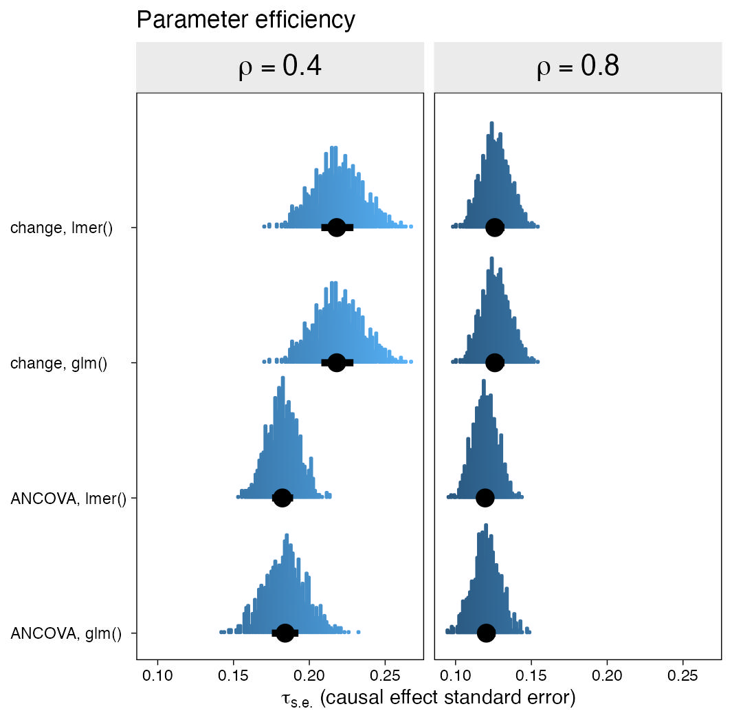
I've been thinking a lot about how to analyze pre/post control group designs, lately. Happily, others have thought a lot about this topic, too. The goal of this post is to introduce the change-score and ANCOVA models, introduce their multilevel-model counterparts, and compare their behavior in a couple quick simulation studies. Spoiler alert: The multilevel variant of the ANCOVA model is the winner.| A. Solomon Kurz